We now get into Nontransitive Dice and Other Paradoxes. If there is a transitive relationship between things labelled A, B and C, then if the relationship holds between A and B, and B and C, then it also holds for A and C. For example, if A is heavier than B, and B is heavier than C, then A is heavier than C. One of the most well-known examples of nontransitivity is the old rock-paper-scissors (or, rock-paper-scissors-Spock-lizard) game.

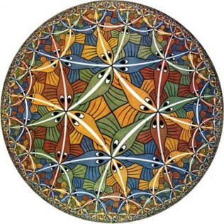
(All rights belong to their owners. Images used here for review purposes only. Efron’s non-transitive dice.)

The above four nontransitive dice were created by statistician Bradley Efron. You allow a partner to choose one of the four dice, and you pick a die from the remaining three, You both toss your dice, and the highest number wins. Even though your partner picks first, you can always find one die from the remaining three that will give you a 2/3’s chance of winning. The reason is that people have a preconceived notion that “more likely to win” is transitive between pairs of dice. In the above illustration, die A beats B, B beats C, C beats D, and D beats A.

Gardner goes on to talk about John Maynard Keynes “principle of indifference” (from A Treatise on Probability) – “If you have no grounds whatever for believing that any one of n mutually exclusive events is more likely to occur than any other, a probability of 1/n is assigned to each.” That is, if you have 6-sided dice that are obviously not loaded or misshaped, each of the faces has a 1/6th chance of coming up on any given throw. With a coin, heads and tails have a 1/2 chance each. The problem is in deciding which events have equal probabilities of happening. Martin gives the following example.

You have a packet of 4 cards, two red, two black. You shuffle them and deal them face down in a row. Two cards are picked at random, such as by putting a coin on the desired ones. What is the probability that both of the selected cards are the same color? One argument is: “There are three equally probable cases: The cards are either both black, both red, or different colors. In two cases, the cards match, so the probability is 2/3.” The second argument is, “There are 4 possibilities, The cards are either both black, both red, or card x is red and y is black, or x is black and y is red. Either they match or they don’t, so the probability is 1/2.” Puzzle for the week: What’s the correct answer?

Or, say you have a covered bucket with red, yellow and blue balls inside, but you don’t know what the distribution is for each of the colors. What are the odds that the first ball you pull out will be blue? Applying the principle of indifference, on the first try, either the ball is blue or it isn’t, so you assign 1/2 to it being blue. Otherwise it will be red or yellow, so the odds for each are 1/4. But if you change the question to what are the odds of the first ball being red, then the probability of getting red first is 1/2 and for blue it’s 1/4, which is a contradiction. The same argument can be used for whether there’s life on Mars or not. The point is that if you don’t know the probabilities for an event, the principle of indifference is going to fail you.

The “most notorious misuse” of this principle was by Blaise Pascal, and is known as Pascal’s Wager. (Taken from the wiki article.)
“”God is, or He is not.” But to which side shall we incline? Reason can decide nothing here. There is an infinite chaos which separated us. A game is being played at the extremity of this infinite distance where heads or tails will turn up. What will you wager? According to reason, you can do neither the one thing nor the other; according to reason, you can defend neither of the propositions…

Yes; but you must wager. It is not optional. You are embarked. Which will you choose then? Let us see. Since you must choose, let us see which interests you least. You have two things to lose, the true and the good; and two things to stake, your reason and your will, your knowledge and your happiness; and your nature has two things to shun, error and misery. Your reason is no more shocked in choosing one rather than the other, since you must of necessity choose. This is one point settled. But your happiness? Let us weigh the gain and the loss in wagering that God is. Let us estimate these two chances. If you gain, you gain all; if you lose, you lose nothing. Wager, then, without hesitation that He is.” In other words, in matters of faith, always bet that the faith holds true. If it doesn’t, you haven’t lost anything (except for all that stuff your faith made you sacrifice along the way.)

The interesting thing is that you can make the same arguments with equal force to any of the other major faiths. And a similar version was written by H. G. Wells in Apropos of Dolores, “While there is a chance of the world getting through its troubles, I hold that a reasonable man has to behave as though he was sure of it. If at the end your cheerfulness is not justified, at any rate you will have been cheerful.”

There’s a lot of reader feedback in the addendum this time, and suggestions for other versions of the nontransitive dice. R. C. H. Chang, from Bath University, England, (at the time), came up with a game using one die. Each face is numbered 1-6, each number is a different color as shown in the chart. The first person picks a color, and the second player selects a different color. The die is thrown, and the person whose color has the highest value wins. Picking the color just to the right of player 1’s in the chart will give you a 5/6 chance of winning.

(The hardware set-up screen.)

I’m pretty much done working with the RoboDesigner kit for the moment, but I do want to get this last write-up done for historical reasons in case I ever come back to this kit later. As I wrote in the last robot blog entry, the programming environment used for the kit, TiColla, that came on the CD-Rom has a few bugs. I was hoping to get under the hood of the save files to see if I could find any work-arounds. I failed on that count, but what I did find kind of helps explain why certain limitations exist the way they do.

TiColla was written by Tairo Nomura, an assistant professor at the University of Saitama. It stands for “TIle COLLAge oriented COLLAborative work environment.” The environment has 3 major screens: Hardware setup, the program workspace, and HTML. The HMTL screen is always empty and apparently not used in this version. The hardware screen is shown above. You drag icons for the different sensors or input sources to the CN1-CN6 connector spaces to represent the actual real-world wiring of the robot.

The two main motors are hardcoded, and the contact switches and IR sensors are intended to go to fixed sockets (CN1 and CN2 are the left and right switches; CN3 and CN4 are the left and right IR sensors). CN5 could be a third motor, and CN6, in normal mode represents PWM (pulse-width modulation) control of the two main motors. However, CN5 and CN6 can also be used as analog inputs for datalogging purposes (I haven’t tried datalogging because I have no use for this with such a simple robot set-up).

(The software workspace.)

The software workspace has four main tabs from which you select the different kinds of icons. Basic gives you motors 1 and 2, motor stop, port (which is only active if CN5 or CN6 are used as inputs) and NOP. Control has Loop, Repetition, Loop/Rep End, Wait, and If statements for status states of the switches, sensors and variables, Yes and No for the If statements, and If for data input levels. Variable lets you do variable initialization (V1-V8), and adding or subtracting values. Finally, Extension lets you program CN6/CN11 for PWM control of the M1 and M2 motors.

The above screen cap shows the line follower program. It starts with Begin Program, then enters a loop. CN3 is the left IR sensor. If the analog out value of the sensor is 20 or below (0-250 allowed), the program takes the Yes branch (Y1), otherwise it takes the No branch (N1). From Y1, we go to the CN4 test for the right IR sensor. If the value is 70 or less (Y2), both motors M1 and M2 will stop (both sensors sense black). From N2, (left sensor senses black, right sensor senses white level), M1 goes backward while M2 goes forward to recenter the robot over the tape. From N1, we go to a second test for CN4, giving us Y3 and N3. From Y3 (left sensor senses white, right sensor senses black), M1 goes forward and M2 goes backward, again to recenter the robot over the tape.

For N3, the robot is already centered over the tape, so M1 and M2 both turn forward. The NOPs are designed to allow reentry of the branches so they remain nested. Lastly, we have End Loop/Rep, and End Program. TiColla has problems handling Repetitions and variables, so I won’t discuss those here.

Most of the tiles have parameters that can be set from the window at the top right. For the motor tile, you can pick M1 or M2; Forward/Backward/Stop/Break; Very Slow/Slow/Mid/Fast; and PWM duty cycle. Wait can be set from 0.1 to 10 seconds. “If” for the contact switches has CN1/CN2; “=1”; and “Numeric”. The analog “IF” for the IR sensors has CN3/CN4; “=<“/”=>”; “Numeric”; and value (0 to 250).

Note that the book claims that the analog IF “gray area” value is 110; anything below that is considered black, and above that is white. But, the photo-transistors aren’t calibrated well, and one is apparently overly sensitive, so I have the left one triggering for “BLACK” if the signal is under 20, and the right one for 70 or less.

This brings me to the actual code. The files are stored in XML format, meaning that we have HTML-style matching <> / </> tags (<timestamp>, </timestamp>, <PortNumber>, </PortNumber>), etc. The code is broken up into major blocks, with a <TIXExchenge></TIXExchenge> wrapper. The first block (<TIXInfor></TIXInfor>) is just version control information.

The second block (<TIXTileSet Name=”project1-PG”>) specifies each of the tiles placed into the workspace. The first object is a special case, in that it’s for “Begin Program” and it sets default operation conditions for the motors (such as exact pulse counts per second for the Slow, Mid and Fast speeds). The general format is:

<TIXTile ObjectID=”1″>
<titleString>
MDRV
</titleString>
<ClassName>
jp.tairo.TiColla.core.TileSet.MotorDriverTileComponent
</ClassName>
<compLocX>
336
</compLocX>
<compLocY>
288
</compLocY>
<connPosition>
2
</connPosition>
<TIXTileMove MotroNumber=”1″>
<Peripherykind>
2
</Peripherykind>
<PortNumber>
8
</PortNumber>
<directionNumber>
1
</directionNumber>
<directionNumber2>
0
</directionNumber2>
<speedNumber>
2
</speedNumber>
<dutyRatio>
50
</dutyRatio>
<breakFlag>
false
</breakFlag>
</TIXTileMove>
</TIXTile>

Explanations:
<TIXTile ObjectID=”1″>: The tiles are numbered in the order they’re moved onto the workspace, and NOT in program execution sequence.

<titleString>: This is the internal name of the icon. For the above example, MDRV refers to motors M1 and M2.

<ClassName>: Another internal parameter, identifying the class code for controlling this part of the program. For this example, it’s the motor driver class.

<compLocX>, <compLocY>: These are the x- and y- coordinates of the icon tile in the workspace (X from the left of the screen, Y from the top). Because the workpace is automatically snap-to-grid, the icons have fixed spacing. This becomes important later for program flow.

<connPosition>: This one’s a bit confusing. It actually represents the location of the tool icons at the top of the workspace toolbar (horizontal straight line is position 1, vertical straight line is 2, etc.) This controls the black line running through the current tile.

The following tags are tile specific. Here, we have the motor tile settings.
<TIXTileMove MotroNumber=”1″>: Motor type 1 block (fixed). Used for both M1 and M2.

<Peripherykind>: Specifies M1 (kind 2) or M2 (kind 24). This tag is also used for Analog IF tiles, in which case the kind is 6.

<PortNumber>: For M1, use port 8; for M2 use port 10.

<directionNumber>: 0 for forward, 1 for backward, 2 for stop.
<directionNumber2>: Always 0.

<speedNumber>: 0 for High, 1 for Mid, 2 for Slow, 3 for Very Slow.

<dutyRatio>: Default is 50.

<breakFlag>: False (no breaks).

——-

IFPA (Analog IF) adds:
<valueType>: 0 = Numeric.
<valueNumeric>: An integer between 0 and 250

——-

WAIT adds:
<value>: A value between 0.1 and 10.

——-

There are a few other tile icon types that have other specific tags, such as VAR and IFPD (digital IF), but those are easy to figure out just by looking at the XML file.

——-

The last XML block is for the hardware setup:
<TIXHardware Name=”project1-HW” HardwareType=”isikari”>

This block lists all possible hardware components, and whether they are specified in the above TiColla hardware configuration screen. Most of this stuff is required for the kit as it is designed, and therefore should not be altered.

Ok, so where is the program flow specified?
That is, how do we know that Begin Program calls Loop, and that Loop calls IFPA for reading IR sensor CN3?

Just by looking at the XML file, we don’t. There are no overt wiring declarations anywhere, either in the workspace screen, or in the XML file.

In fact, program flow is determined implicitly based on tile locations. This is where the snap-to-grid feature comes in. The icons all have fixed heights and widths, and flow starts from the bottom side of the Begin Program (BGNP) icon. It goes to the next icon in the same column (compLocX = 384), but one icon height (48 pixels) down, which is the Loop tile. The next icon below Loop at compLocY = 96 is the analog IF tile for IR sensor CN3.

This IFPA tile has connPosition 8, which is a sideways “T” intersection pointing to the left. The “Yes” tile for this IF is at compLocX = 336, compLocY = 96. The “No” tile is compLocX = 384, compLocY = 144.

And this is where I think TiColla runs into problems with long strings of icon instructions – it just can’t keep track of the ends of Loops and Repetition statements; and non-nested branches confuse it even further. Additionally, there may be an array limit for storing all of the tile blocks, causing a possible array overrun.

—————-

Overall, I think TiColla was a nice concept, but choosing XML for the data structure was a mistake. (My buying the kit 2 years after software support for TiColla ended was ill-timed, too.) The kit is fun to play with, but it has its limitations. I’ll keep it and pull it out of the box occasionally to make more elaborate black tape maps for the line follower.

Wednesday’s answer for the probability puzzle:

When the warden talked to prisoner A, the chances of picking any one of the prisoners as not having been pardoned was 1/3, so that didn’t affect A at all, and his odds of surviving are still 1/3. But C’s chances go to 2/3.

Gardner’s proof:
1. C is pardoned, warden names B (probability 1/3)
2. B is pardoned, warden names C (probability 1/3)
3. A is pardoned, warden names B (probability 1/6)
4. A is pardoned, warden names C (probability 1/6)

Only cases 1 and 3 apply when B is named to die. The chances that it is case 1 are 1/3, or twice the chances that it is case 3, so C’s chances of survival are 2 to 1, or 2/3.

However.

Marilyn vos Savant ran a Monty Hall “Let’s Make a Deal” version of the prisoner’s problem in her Sept. 9, 1990, column in Parade magazine. Say Monty has a contestant that has a choice of three doors. Behind one of them is a car, and behind the other two are a pair of goats. The contestant picks one door (odds 1/3) and Monty then has one of the other doors opened to show a goat. If the contestant now switches their choice to the remaining door, their odds of getting the car jumps to 2/3. That is, if the first door had a 1/3 probability of being right, eliminating one of the wrong doors means that the probability with the remaining unopened door has to add up to 1, and therefore door 3 has a 2/3’s chance of actually having the car.

We now get into Probability, with the chapter on Probability and Ambiguity. Say you have 3 coins and your friend has 1. You throw all three, and he throws his three times in a row. What are the odds of both of you getting three heads? The answer is that both of you have the same odds, but not all mathematicians in history would have accepted that. The point is that probability theory gives clear answers, but only if you word the experimental procedure precisely.

What if you have a long stick and you break it randomly into three pieces, what is the probability that the pieces can be put together to make a triangle?

(All rights belong to their owners. Images used here for review purposes only.)

One approach is to pick two points independently along the range of the stick, and then break it at those points. The answer is then 1/4. The proof is given above. Draw an equilateral triangle with an altitude the height of the stick. Connect the midpoints of the triangle to make a smaller, gray, triangle. Pick any point within the larger triangle and draw segments perpendicular to its sides. The sums of these segments will always equal the altitude. If the point is in the gray triangle, no one of the segments will be longer than the sum of the other two, and the three of them will form their own triangle. Otherwise, if the point is outside the gray area, one segment will be too short. And, that gray region is 1/4th the area of the larger triangle as a whole.

But, if we reword the procedure, we could take the stick and make the first break. We randomly pick one of the two pieces and make the second random break. What are the odds now? If we pick the smaller of the two pieces to make the second break, we can’t make the triangle. If we pick the larger piece, it must not be so long as to reach the smaller space above the gray region of our picture, limiting the second break to the other 3 regions, for odds of 1/2 * 1/3 = 1/6.

A second example was posed by French mathematician Joseph Bertrand. What is the probability that a chord drawn at random inside a circle will be longer than the side of an equilateral triangle inscribed in the circle. Approach one – start from some point on the circumference of the circle. The other end ranges uniformly over the circumference, making an infinite number of equally probable chords. Only the chords that cut across the triangle will be longer than its side. The angle of the triangle at A is 60 degrees, and the possible chords lie within an 180 degree range, the chance of drawing a long enough chord will be 60/180 = 1/3. (Top illustration.)

Approach two – The chord drawn must be perpendicular to one of the circle’s diameters. Draw the diameter, add the triangle. (Bottom right illustration.) All chords perpendicular to the diameter will pass through a point ranging uniformly along the diameter. Set point A at the center of the bottom of the triangle. The distance from A to the center of the circle is 1/2 the radius. B is the midpoint on the other side of the diameter. Only chords crossing the diameter between A and B will be longer than the side of the triangle. AB is one half the diameter, so our answer is 1/2.

Approach 3 (bottom right illustration) – Draw a smaller circle inscribed within the triangle. Draw the chords from one side of the larger circle to the other. Only chords whose midpoints lie within the smaller circle will be longer than the side of the triangle. The area of the smaller circle is 1/4 of the larger one, so the odds are now 1/4.

Which approach is correct? Well, it depends on what your definition of “is”, I mean, “draw a random chord” is.

Then we get the following problem. In a prison, there are three prisoners that have all been sentenced to death, and are kept in separate cells. The Governor decides to pardon one of them. He writes their names on three slips of paper, put the slips into a hat and pulls one of the names. He calls the warden and tells him the name of the lucky guy, requesting that the warden keep it a secret for several days. Prisoner A hears a rumor about this, and tries to get the warden to tell him who was pardoned. The warden refuses, so the prisoner says, “Then give me the name of one of the other men who will be executed. If B has been pardoned, say “C,” and if it’s C, give me B’s name. Otherwise, flip a coin to name B or C.” The warden leaves, thinks about this overnight, and the next morning tells A, “B will be executed.” The warden leaves again, and A is happy, because his odds went from 1/3 to 1/2. He taps on a waterpipe to prisoner C and instructs him to ask the exact same question to the warden. The warden gives him an answer, and C is also happy because his odds also went up to 1/2.

Puzzle: Did prisoners A and C ask the right questions?

Addendum: Gardner discovered that his second version of the broken stick problem was worded wrong. He’d taken it from William Whitworth’s “DCC Exercises in Choice and Chance,” and it was completely incorrect. Skipping the math, the correct probability 1/2 * (-1 + 2*log(2)) = 0.193, which is just a bit larger than Whitworth’s answer of 1/6.

Ok, so I have the RoboDesigner robot kit sitting back in its corner, and I’m trying to decide what to do with it next. The contact switches work for the wall avoider program, and I can run simple patterns with it (like spike snowflakes and pentagrams); but neither of the two IR sensors work, which nullifies 2/3rds of the programs in the instruction book, such as the line follower. I’ve double-checked the wiring of the LEDs and jumpers, and verified all the instructions in the book several times. I’m close to taking the IR sensor boards off and mailing them to someone that has actual diagnosis tools, but I’m not quite at the breaking point, yet.

(The robot with the lower form factor.)

I do have a semi-useful voltmeter buried in a box in a different corner, and one day I have just enough free time on my hands that I finally dig the thing out and clean all the mold off it (this is Japan, and we have a humidity issue here…), which is another reason why I’d been holding off on retrieving it. I verify that the meter still works, and that both IR sensor boards are getting power via the ribbon cables. However, it turns out that one of the two LEDs has an open path leading up to it, and, after looking at the solder jumper REALLY carefully, I notice that it’s not actually making contact with one of the jumper pads. I re-re-re-solder the jumper, and I measure about 2.5V across the LED. I check the second board, and there’s a 2.5V drop on that LED, too. There’s no visible indication when the IR LEDs are active, so I plug the cables into the sensor board sockets and aim the LEDs at the photo-transistors of their sister boards, while running a test program (each sensor controls one motor, if the sensor turns on, so does its associated motor) and they both work.

This confuses me, because neither board had worked before, and I only found one problem on one of them (the jumper), so why wasn’t the other board working either? I put reflective paper in front of the sensors so they’ll trigger themselves, and the second one doesn’t trigger this time. Messing around with that one some more, I realize that the photo-transistor sensitivity is way off, and the board has to be recalibrated. I adjust the offset pot. by 50%, and now both sensors trigger with the reflective paper at about the same distances.

Pushing my luck, I tape 6 sheets of printer paper together and lay down a simple loop path with black electrical tape. I load the line follower program into the robot, and the thing kind of reacts to the black tape, but not very well, and it keeps wandering off the paper. So I wrap black tape around the sensor boards (as suggested in the book) to isolate the LEDs and photo-transistors from each other, and I tinker with the program settings. I remove wait times, and instead of stopping one wheel while the other one turns when one of the sensors senses the tape, I have the stopped wheel moving backwards at the same time. Plus, I have to readjust the good sensor pot. to make it less sensitive, too. After about an hour of all this, I have the robot actually following the tape loop correctly. Yay me.

But, this is boring. I want the contact switches involved as well, and I want the robot to recognize obstacles along the loop, and broken loop paths. That means loading the “rescue robot” program, and implementing the more sophisticated problem handling routines in the book. I’d already typed these routines up, so all I need to do is download them to the robot. I try doing this thing, and the PC software (named TiColla) locks up.

I stop the download and try again. TiColla locks up again. I close TiColla and reopen it – same problem. I check the cables, the switch settings on the robot, etc., same thing. I reboot the PC, disconnect the cables, reconnect them, try again, TiColla still locks up. I already know that the program for the “dance robot” won’t compile, and I’ve had similar compilation issues with some custom programs I’ve written that just use the contact switches, so I assume that maybe the problem now is inherent in the rescue robot program. I reload my line follower, and that downloads to the robot just fine. Which leads me to think that there’s possibly a memory limitation in TiColla. Unfortunately, TiColla came out in 2004, and is no longer supported. In fact, I can’t find a newer version on the existing website at all. My only option is to try keeping the programs small.

I don’t give up yet, though. I save the line follower to a new file and slowly add elements to it so the robot will back up if it hits something, and then to turn 15 degrees to either side depending on which switch is hit, before going forward again. This part works. All that’s left is to try having the robot go in an arc around objects, and this is really where TiColla disappoints. There are two tile icons, one for doing a specified number of repetitions, and the other for making decisions based on setting and testing variables. Nested repetition loop program examples given in the book don’t compile, and variable handling seems to be what causes the downloader to lock up. I’ve already encountered 5-6 mistakes in some of the other programs in the book (like in the wall avoider and the line follower), so I’m not surprised to uncover bugs in TiColla. I’m guessing that these bugs were fixed at some point, but the author dropped online support for TiColla in 2014, and all I have left is what came on the CD-ROM with the kit.

So, I try incorporating the full wall avoider in with the line follower, and the robot gets really wonky. I still want the robot to go around physical obstacles, which should be easy if I just hardcode the routine I want (back up, turn 45 degrees, go forward 1 second, turn 45 degrees the other way, go forward 2 seconds, turn 45 degrees again, go forward 1 second, turn 45 degrees the other way, resume path). But when I try this, the contact switches stop working and the robot’s movements become unpredictable. I strip the program down to just the avoider, and same problem. So I start from scratch and just build the avoider up in stages, and it seems there’s a length limitation for how many motor actions I can have in one sequence. When I get to 12-15 tiles in one string, the branching logic for the contact switches stops working. Sigh. So I go back to the line tracer, and just add a simple “stun” reaction (if a contact switch is sensed, back up 0.5 seconds, then sit still for 2 seconds to let someone remove the obstacle before continuing forward. That works, and is actually kind of cool-looking.

Anyway, the line follower works, the IR sensors work, and I can incorporate the contact switches in with the follower. Any other programs I want to write, such as logo turtle-style patterns, light avoiders, and even stuff using custom sensors, can be treated as smaller, single-purpose stand-alone programs. I am contemplating removing the controller and RS-232 boards, keeping the motor driver, and wiring in my old Arduino board instead. But, that’s a project for the far future (assuming that I don’t simply buy a new integrated robot kit at that time).

I rest (mostly) happy now. Also, I made a couple videos of the line follower at work (below).

(The sensor boards as viewed from below. The photo-transistors are the little black rectangles directly above the LEDs.)

Actually, after I’d gotten everything working, and had settled on the finished line follower program, a strange thought occurred to me. The IR LEDs used with this robot kit are very much like the ones used in TV remotes. So, what would happen if I aimed a remote controller at one of the photo-transistors when the robot was running the line follower program? I try this thing, and the motor associated with that transistor turns on briefly (the signal from the remote only lasts a fraction of a second). I try again, the motor turns on briefly again. Cool. I try a second remote, for the air conditioner, and again the transistor sees the infra-red signal from that controller. Then I get a really weird thought – digital cameras sometimes use IR for measuring distances to the subject for focusing the lens. What would happen if I aimed my pocket camera at the IR LEDs while the robot was turned on? Sure enough, there was a faint purplish glow on the view screen, which was not visible to the naked eye (see above photo). Now I have hard confirmation that the LEDs really are emitting infra-red. Mucho cool.

Direct youtube link

Answers:

Unknotting a 2-holed torus.

Having one torus eat another.

Removing one toroid hoop from another toroid.

Doughnuts: Linked and Knotted

Before I get started on the Gardner chapter, I want to put down some thoughts here on topology. I had never really heard about topology as a field of mathematics when I was in school, and it wasn’t until maybe the mid-1980’s that I encountered the whole doughnut-coffee cup equivalence thing. But, in the last year, I’ve been running into it more often, in the writings of George Gamow and Martin Gardner. One reason for topology attracting a physicist’s attention is in its relationship to Einstein’s statement that space is warped. If this statement is indeed true, then topology can possibly help explain what the universe really looks like to an outsider (i.e. – someone standing outside our universe).

(All rights belong to their owners. Images used here for review purposes only. Escher’s Circle Limit III.)

At the same time, though, we have M. C. Escher’s Circle Limit III woodcut (blog entry #14), which illustrates what a hyperbolic universe could look like. Again, within that universe, the lengths of the fish are all the same, it’s just that you the inhabitant, and all your measuring devices, get proportionately smaller as you get closer to the rim of the disk. So, think about that – if space is warped, and anyone living within that space gets warped simultaneously, you can’t tell through direct measurements that anything is going on because your rulers warp, too.

Ok, why bring this up? Because gravity is not a force, it’s a side effect of mass. If mass warps space, and space remains “flat” in the absence of mass, then the contraction of space around a point centered within a given mass can be thought of as being like the reciprocal of the hyperbolic world of Circle Limit III. Things get smaller as you get closer to the center of the “disk.” What we call “gravity” then is the result of this warping, where the distances between three adjacent parallel (from our perspective) lines (in my above figure, say three vertical lines running through x = 1, 2 and 3) aren’t equal. The energy then to go in one direction is not the same as for going in the opposite direction because the spacing between the lines is smaller in one direction than in the other. This warpage is perceived as gravity only in that we have no other way of seeing what is happening to us at this scale. The farther away we move from this mass, the less differential in distances between adjacent parallel lines, and less “pull” to the center of the mass that we experience. “Weightlessness” is where the “real” distances between three adjacent parallel lines are more or less equal. To an outside observer, people within pinched space would look smaller than they would when “weightless.”

One reason I don’t like the traditional drawings of gravity wells is that they’re shown in polar coordinates around the mass, as if there really is a gravity “well” (or energy hole) of some kind. I think a pinched rectangular grid would be a better choice, especially if you animate two or more masses (like two orbiting black holes, or our Earth and moon orbiting the Sun). You’d be able to visualize gravity waves better this way, I’d expect. If I ever figure out how to draw this kind of animation, I will. Anyway, the problem with developing a Grand Unified Theory is not one of figuring out how to relate gravity to the weak and strong forces, but how to tie the distortion of space via a charge-neutral mass to those other charged forces. M-Theory, and the application of 10-, 11-dimensional space might not be that far off. (Yes, I know my ideas are not original and/or new. But, they are mine.)

(Making a torus by rotating a circle around an axis.)

Ok, so, doughnuts to you. Martin begins by introducing the torus as a circle rotated around an axis that doesn’t intersect the circle, and he draws parallels with coffee cups, rubber bands and a sphere with one handle. He then mentions that a rubber model of a surface cannot be deformed in 3D space to make ALL topologically equivalent models. That is, a Mobius strip has a “handedness” that you can’t alter through stretching and twisting. This “handedness” disappears in 4D space, though.

After talking about turning a torus with a hole in it inside out, Martin continues to the idea of tori with knots tied into them. The above illustration shows the two types of trefoil knots possible – an outside knot, and an inside knot. One way of visualizing the inside knot is to take a wood block and drill a hole through it in the knot shape. He adds that it is not possible for a torus to have both an inside and outside knot, which would be similar to the pseudo knot at the above right. Untying the outer knot simultaneously unties the inner knot, showing that the model is topologically identical to an unknotted torus, elongated to look like a garden hose.

R. Bing wrote a paper in 1965, entitled “Mapping a 3-Sphere onto a Homotopy 3-Sphere,” where he showed that the top right cube with a hole (fig. 20.4) and a second hole knotted around it is topologically the same as the top left cube with two straight holes (fig. 20.4). Because in this system the end points of the holes can be moved around easily, the solution (fig. 20.5) is to first deform the right side hole to look like a single line (mainly to make the proof easier to follow), then run one end of the hole up the side of the other one, around the top of the cube, and then along the side and back to the bottom.

We then get examples of two-hole tori, and there are a lot of varieties of these.

The addendum talks about intrinsic and extrinsic properties of a surface, and states that the two above surfaces are equivalent. There’s a lot here if you’re interested in topology, so it’s either better to buy the book, or refer to the wiki article.

Puzzles for this week:

Can you untie the below left torus to get the figure on the right?

Almost 1 year ago, I wrote about building a RoboDesign Kit robot, from Cutt. At the time, the main problem I had was in getting a cable to connect my laptop to the robot. The kit was designed for a 9-pin serial cable running from the COM ports, and modern PCs don’t use COM ports anymore. I asked for a 9-pin serial to USB converter cable from home (couldn’t find anything like this in Japan) and received the 6′ cable from D-Tech in December. The next issue was whether I’d be able to get updated software from TiColla, but that turned out to be a dead end, since the kit came out in 2006, and the software isn’t supported anymore.

(TiCollo hardware assignment screen.)

So, I dither about a lot, and then I get distracted, and then I have a lot of books from Christmas to read, including the Crypto Contest book and Martin Gardner’s Colossal Book of Mathematical Puzzles, and time just slips by me. Finally, before my birthday, I knuckle down and break out the kit manual again. I install the programming software off the CD, plug in the USB adapter cable, and see what I’ve got. Amazingly, the CD-ROM software runs right away, the cable driver is recognized and installed, and the robot itself turns on (after I run to the 100 yen shop to buy 4 C-cell batteries). With nothing better to do, I set up the TiCollo environment so the robot is configured to know that it’s got the 2 DC motors and 2 contact switches, then I move the icons around to create a short test program to turn on one motor for 1 second. I set the switches to download the program to the robot, turn it on, and click “send.” The LEDs on the board don’t flicker, but TiCollo says the program downloaded. I turn the power switch off, change the second switch to “run program,” turn it back on, and press the “go” button.

(TiCollo’s programming environment is icon based.)

Nothing. I try again. Nothing. I change the switches and try again, and the robot jerks forward a bit then turns off. I change the program again, but I get the same jerky motion. I keep messing around with the switches, checking the connections, and even trying more complex programs, but the robot seems crippled somehow. Finally I decide that the kit is broken and I did what I could do with it. It was fun to build, but I’d hadn’t gotten my hopes up that it would still be functional after so long. Great, time to put it out for recycling.

More time goes by. I get more books for my birthday, and that keeps me REALLY busy through August. But, when I get to the Prolog Programming book, I feel frustrated. Prolog is interesting, but I can’t find the kind of AI example programs I was hoping would be online, and the examples I do find are for other flavors of Prolog that don’t run under Gnu-Prolog without massive rewrites. I spend a week learning Prolog, then have nothing that I really want to use it for. I’d thought about trying my hand at playing with symbolic logic as described in the Smullyan book on the Godel incompleteness theorem, but I really need examples to work from, and I can’t find anything.

So, I put the Prolog book away, and I return to the idea of cleaning out stuff from the apartment to make more room, bringing me back to the robot still sitting in its little corner. And there are two things still bugging me about it. The environment software kept defaulting to 9600 baud when transmitting the program to the robot, and I’d been wondering if that speed was too high for the cable. To check, I bring the robot and cable back out, hook everything up, and run the TiColla software again. The only option in the send screen is to deactivate 9600 baud mode, but I have no idea what that means. I send the program – no change from before. That leaves the second thing – 9-pin serial cables often had the send and receive pins cross wired. I don’t know if my USB adapter cable is cross wired or straight through. And I don’t have any way of checking. Before I give up, though, I start inspecting all the switches and jumpers on the microcontroller board to see if I can find any clues. And, stenciled next to one switch on the interface board, I read “Cross” – “Straight.” It’s currently on straight, so I set it to cross and try downloading the test program one more time. And what happens? The LEDs flicker madly, and when I press the “go” button, the robot goes exactly the way its supposed to go. I load the obstacle avoidance program, run the robot, and watch as it backs up and goes in a new direction when the feeler switches get bumped.

Well. I now have a choice. I can either throw the thing away like I’d been planning to, or I can make it do tricks. Decisions, decisions…

Actually, I’d hadn’t soldered in the infrared LEDs to the sensor interface boards, or attached those to the the robot frame yet. Those are needed for the bulk of the programs in the book, so I take care of that, which takes about 15 minutes, mainly because of how the hardware is designed to mount the front “bumper” to the main frame. Then, I write up a small program to test the IR sensors, and that doesn’t work. The LEDs are supposed to be infrared, so presumably you can’t visually tell if they’re on. But, I found a photo of the kit online, and that showed the LEDs as glowing bright blue, which bothers me (if IR LEDs had a visible component, it would be reddish, so I suspect the glow was photoshopped in). Then I go back to the book again, and discover a separate wiring instruction stating that to use the LEDs, you need to solder a jumper point on both boards. I do that, and still no change. I mess with the kit a lot more, and it seems that one of the two photo-transistors is more light sensitive than the other one, which gives me hope that by changing the potentiometer settings I can get them to be equally light sensitive, and that works a little bit. I tape sheets of printer paper together and lay down a track with black electrical tape, and the line follower program recognizes the tape just enough to be teasing, but the tape apparently is too glossy, and the photo-transistors generally can’t tell the difference between that and the paper.

Finally I give up and go back to just playing with the motors, loops, and contact switches. Then I run into a limitation in TiColla, which keeps flagging me if the program gets too long. That’s bizarre, because there are longer programs in the book for the soccer playing robot (which requires a plastic soccer ball with IR LEDs inside, so I can’t use the robot in actual play because I don’t have the IR ball, or a second robot to act as a goalie). I assume the problem is in the software, which I can’t update. Now, yeah, I have to give up and say that I had a better run with this kit than I’d expected. I still have the wall avoider, and I can write limited logo turtle-style pattern runners. I’ll show the kit off to my students, and move on to the next distraction.

Just as a side note, the maker of the kit, Japan Robotech, still has a website presence, and their current machines are built around the Arduino.

Treat the above knot as one piece of rope with no loose ends. Move the ring from the bottom knot to the top one without untying the rope. (The solution is in fig. 19.9.)

Knots.
Have you noticed that I often start out with “Gardner starts out by saying…”? No? Maybe I shouldn’t have mentioned it. Anyway, Gardner starts out by saying “To a topologist knots are closed curves embedded in three-dimensional space.” The knot is defined as “trivial” if you can model it projected on a plane as a curve with no crossing points. That is, the curve is not knotted. “Links are two or more closed curves that can not be separated without passing through one another.” Gardner also makes mention of Lee Neuwirth’s The Theory of Knots (1979, Scientific American). Most of the math in this chapter can be found in the wikipedia article, so I’m not going to repeat it here.

(All rights belong to their owners. Images used for review purposes only. Three examples of nonalternating knots with 8 crossings.)

First, though, knots can be classified by the number of their crossings, and whether they are alternating or nonalternating. That is, if you follow the knot along the string in one direction or the other, the string will alternate going over and under at the crossings. Nonalternating knots don’t alternate. You can also divide them as prime or composite. A prime knot can not be manipulated to make two or more separate knots. Gardner gives the square and granny knots as examples of composites, because they can be changed to two side-by-side trefoils. The square knot is a combination of two trefoils of opposite handed-ness, and the granny is the product of two trefoils of the same handedness. Both are alternating. Gardner challenges the reader to diagram a square knot with 6 alternate crossings (the minimum).

(A two-strand braid that goes around two “holes”.)

Knots can also be invertible and noninvertible. That is, paint an arrow on a knotted rope to give the curve a direction. If you can manipulate the rope to keep the same structure but the arrow pointing the other way, the knot is invertible. According to Gardner, all knots of 7 or fewer crossings are invertible, as are all but one 8-knot and four 9-knots. Hale F. Trotter released a paper in Topology, 1963 titled “Non-invertible Knots Exist”. Trotter discovered an infinite family of pretzel knots that don’t invert – pretzel knots can be drawn on the surface of a two-hole torus without any crossings. An example is given above.

The figure here is of the simplest noninvertible knot, an amphicheiral 8-knot, proved by Akio Kawauchi in 1979. (Amphicheiral means that it can be manipulated into its mirror image.) It is the only noninvertible 8-knot.

The addendum talks about all the new advances in knot theory since his article originally ran in 1983. One of the big discoveries was that certain knot concepts (specifically the Jones polynomial) could be understood in terms of statistical mechanics and quantum theory. For more information, check out Journal of Knot Theory and Its Ramifications.

Finally, the puzzle:
Treat the above knot as one piece of rope with no loose ends. Move the ring from the bottom knot to the top one without untying the rope.